Unlocking the Power of Predictive Analytics

This blog takes you on a journey of exploring the world of Linear Regression. Through the use of a simple yet powerful example of hours studied and scores data, we dive deep into the workings of this popular machine learning algorithm. From understanding the basics of linear regression to its implementation and evaluation, this blog provides a comprehensive guide to help you master the art of making predictions using linear regression. Get ready to unlock the secrets of this algorithm and take your machine learning skills to the next level!

Linear Regression is one of the simplest yet powerful machine learning algorithms that help us make predictions based on a linear relationship between two or more variables. The basic idea behind this algorithm is to establish a relationship between a dependent variable (output) and one or more independent variables (inputs). This relationship is established through the best-fit line that represents the relationship between the variables.

In simple terms, linear regression tries to find the line of best fit that describes the relationship between the input and output variables. The line of best fit is determined based on the minimum distance between the actual values and the predicted values. This line of best fit is used to make predictions on unseen data.

Let's take a look at an example to understand linear regression better. Suppose we have a dataset that contains the number of hours studied and the scores obtained in a test. The goal is to establish a relationship between the number of hours studied and the scores obtained and use that relationship to predict the score for a given number of hours studied.

To implement linear regression, we start by plotting the data on a scatter plot. The scatter plot helps us to visually represent the relationship between the input (number of hours studied) and the output (scores obtained).

Next, we fit a line of best fit to the scatter plot. This line represents the relationship between the input and output variables. The line is fitted in such a way that the distance between the actual values and the predicted values is minimized.

Next, we fit a line of best fit to the scatter plot. This line represents the relationship between the input and output variables. The line is fitted in such a way that the distance between the actual values and the predicted values is minimized.

Once the line of best fit is established, we can use it to make predictions. For instance, if we want to predict the score for 6 hours of study, we can simply use the equation of the line and substitute the value of the input (6 hours) to get the predicted score.

The prediction made using linear regression may not always be accurate. To evaluate the accuracy of the model, we use a metric called Root Mean Squared Error (RMSE). RMSE is the square root of the average of the squared differences between the actual values and the predicted values. The lower the RMSE, the better the model is at making predictions.

Now that we have a basic understanding of linear regression, let's move on to its implementation. Linear regression can be implemented in Python using various libraries such as scikit-learn, statsmodels, etc.

Here is an example of implementing linear regression in Python using the scikit-learn library:

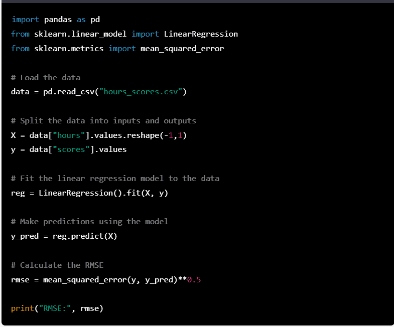
In this example, we start by loading the data into a pandas dataframe. We then split the data into inputs (hours) and outputs (scores). The LinearRegression class from the sklearn.linear_model library is used to fit the linear regression model.

You can download the dataset from here

This dataset contains the number of hours studied and the corresponding scores obtained in a test. The goal is to establish a relationship between the number of hours studied and the scores obtained and use that relationship to predict the score for a given number of hours studied.

R Squared, Adjusted R Squared, and Root Mean Squared Error (RMSE) are commonly used metrics to evaluate the performance of a linear regression model. Let's take a look at each of these metrics in detail:

1. R Squared: R Squared (also known as the coefficient of determination) is a measure of how well the regression model fits the data. It represents the proportion of the variance in the dependent variable that is explained by the independent variables. R Squared ranges from 0 to 1, with a higher value indicating a better fit of the model to the data.

Example: Suppose we have a linear regression model that predicts the price of a house based on its square footage. The R Squared value of this model is 0.8, which means that 80% of the variance in the house prices can be explained by the square footage.

2. Adjusted R Squared: The R Squared value may increase even if a new variable is added to the model, even if it has no effect on the dependent variable. The adjusted R Squared takes into account the number of independent variables in the model and adjusts the R Squared value accordingly. It is a better indicator of the model's fit to the data compared to R Squared.

Example: Suppose we add a new variable "number of bedrooms" to our previous example of a linear regression model that predicts the price of a house based on its square footage. The R Squared value of this new model may increase, but the adjusted R Squared may decrease, indicating that the new variable may not have a significant effect on the model's performance.

3. Root Mean Squared Error (RMSE): RMSE is a measure of the difference between the actual values and the predicted values. It represents the average error in the predictions made by the model. The lower the RMSE, the better the model is at making predictions.

Example: Suppose we have a linear regression model that predicts the sales of a product based on its advertising budget. The RMSE of this model is $1000, which means that on average, the predictions made by the model deviate from the actual sales by $1000.

In conclusion,

R Squared, Adjusted R Squared, and RMSE are important metrics that help us evaluate the performance of a linear regression model. By using these metrics, we can determine how well the model fits the data, how well it makes predictions, and make improvements to the model accordingly.